Multilayer Model in PyTorch
In our last article, we talked about the basics of PyTorch and Deep Learning, now let’s get a little deeper.
Summary:
1- Remembering Deep Learning basics
2- Creating a basic model using PyTorch own classes
3- Creating a multilayer model
4- Using GPU
5- Conclusions
6- References
1. Remembering Deep Learning basics
Model
A model have parameters, the parameters are weights and biases. Parameters do operations with the input.
The linear layer is one of the most basics layers that a model could have. This is the linear layer equation:
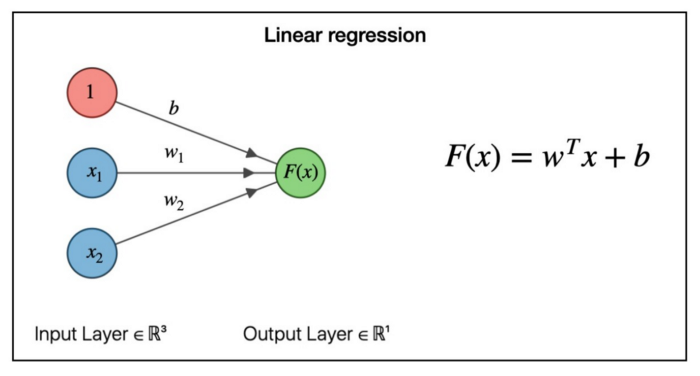
For the linear layer, the weights size is (target_matrix_size X input_matrix_size) and the bias is the target size.
We use a loss function to calculate the difference between the model output and the actual target.
Loss Function
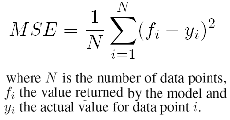
One of the most commonly used loss functions in Deep Learning is the MSE (Mean Squared Error)
Optimizer
Why do we need to optimize the model?
We need to use an optimizer to adjust the model weights and biases to approach the data graph line.
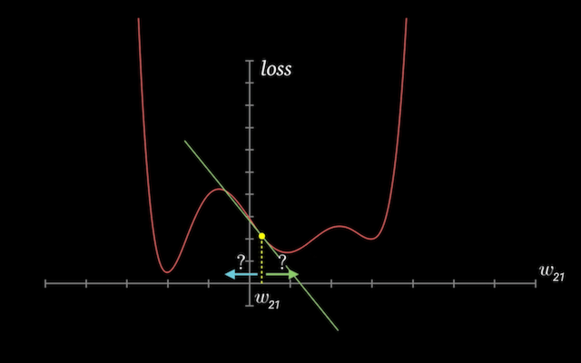
To improve the model, we use the loss to calculate the derivatives of the loss by the parameters, because when we get the tangent of the loss graph, we can adjust the model to have the smaller tangent, and then we will have the smaller loss.
So we just subtract small quantities of the parameters using the gradient value little by little.
If the gradient is positive:
- increasing the weight element’s value slightly will increase the loss
- decreasing the weight element’s value slightly will decrease the loss

If a gradient element is negative:
- increasing the weight element’s value slightly will decrease the loss
- decreasing the weight element’s value slightly will increase the loss
Training the Model
And finally, for training the model, we must follow 5 steps:
- Make predictions
- Calculate the loss
- Calculate the gradients
- Adjust weights and biases
- Reset parameters grad
And is basically these 5 steps repeating for a couple of times to train the model.
2. Creating a basic model using PyTorch own classes
First: Let’s import the data.
In this model, we are going to use the MNIST dataset, that is dataset that contain 60k images of handwrite number from 0 to 9.
We will create a dataset and a data loader that will load the data in batches of images to the model, because if we load all the images in the model at the same time… well, probably your computer won’t handle a big quantity of data in memory
Second: We will create a basic model but using PyTorch class Module for models.
If you don’t understand very much about classes in Python, I recommend you to read this page: https://www.w3schools.com/python/python_classes.asp
So, in the model will enter a tensor with the size (batch_size, 1, 28, 28) and will return a tensor of the shape (batch_size, 10), because the input image will be a number between 0–9, and the model should return an array of probabilities of what number the input should be. Ex:
[0.1, 0.034, 0.34, -0.2, 0.04, 0.1, 0.02, 0.04, -0.1, 0.5]
This array is saying that the input number should be 9, because the biggest probabilitie is 0.5, and we just want the biggest number index, and our index in this case is 9
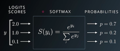
Third: So, now we can convert the numbers of the array to probabilities. We will use a simple equation called Softmax.
Fourth: Let’s define the accuracy function to check model performance.
Then, we need to define the loss function and the optimizer.
For the loss function, we are going to use the Cross Entropy, because the accuracy is great for us humans to see how many the model is performing, but for a computer, accuracy doesn’t show the difference between the predictions and the targets.
It’s not a differentiable function.
torch.maxand==are both non-continuous and non-differentiable operations, so we can't use the accuracy for computing gradients w.r.t the weights and biases.It doesn’t take into account the actual probabilities predicted by the model, so it can’t provide sufficient feedback for incremental improvements.
Explanation took from: https://jovian.ai/aakashns/03-logistic-regression
We just pick the number index of the output array that is equal to the target and apply logarithm. If the probabilities is close to 1, so more close to 0 will be the loss, if the probabilities is close to 0, bigger will be the loss, because we multiply the result by -1.
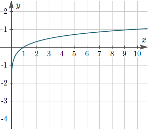
We just took the average of the cross entropy.
And we don’t need to pass the data to the softmax function before the cross entropy.
For the optimizer, we just use the SGD that we learned on the previous article (gradient descent).
Fifth: For the final, let’s train the model.
Just follow the 5 steps that we saw on the previous article.
The model will get an accuracy of 90% in more or less 30 epochs.
We can make it better adding a hidden layer to the model to learn non-linearity.
3. Creating a multilayer model
To create a model with a hidden layer, actually, is very simple. You just need to pass the data to the next layer after the previous layer, but you need an activation to make the model non-linear.
We will use the ReLU activation for the model. The ReLU just take the values higher or equal to 0, and the negatives values set to 0.
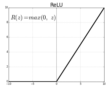
I recommend you read this article to learn more about when to use activation function: https://machinelearningmastery.com/choose-an-activation-function-for-deep-learning/
A good hidden size is between 32–256 parameters. You can choose the size, depends on your model.
Now if we train the model, the model gets 90% of accuracy faster than before. But our model performance time while training is slower than before. This is because the computer requires more computation.
So let’s use a GPU to make the training faster.
4. Using GPU
First we need to get the GPU if the computer have one
device = torch.device('cuda' if torch.cuda.is_available() else 'cpu')Then we pass the model to the GPU just using .to(device)
model = MNISTmodel(in_size, hidden_size, out_size).to(device)And we adjust the train loop to add the tensors to GPU on the beginning.
To pass the tensors to GPU, we pass it to the CUDA, because CUDA is a platform for developers in GPU.
Now let’s train the model again to see the performance.
As you can see, the training is faster than before.
Here are the full code:
5. Conclusion
Cross entropy is good for our model because we are dealing with probabilities, and MSE wouldn’t work very well in this case.
As we see, it is better to use a hidden layer and an activation function to add non-linearity to the model. You can add more hidden layers to the model if you want to make it more powerful, I recommend you to play with this model and try changing the batch size, the learning rate, epochs, optimizer, add more hidden layers… and try changing the hidden layer parameters size.
For the next article, we will improve this model using convolutional layers.


